Revenue Forecasting using Machine Learning
I recently got my hands on a large financial dataset of stocks traded a U.S. exchange. The dataset spans over 30 years (1996 to 2017) and 1949 securities. This is a so-called “panel” dataset, meaning there are multiple snapshots of available historical data for multiple given snapshot dates, called as_of_date. For each as_of_date, the panel includes financial data of companies over the past 24 updates (one update every quarter for up to the past 6 years, labeled by the datadate). These represent the most recent financial statements available as of that point in time.
To see the full jupyter notebook (as html) used for this analysis, click here.
Note: I intend to re-do this project in the near future using freely available data.
1. The dataset
The first challenge is dealing with the large dataset, which occupies ~3 Gb of live memory. However, inspection reveals that there is a lot of quasi-duplicate data. This is the nature of financial panel datasets, where data from a given date (datadate) appears in multiple different snapshots (taken at the as_of_date).
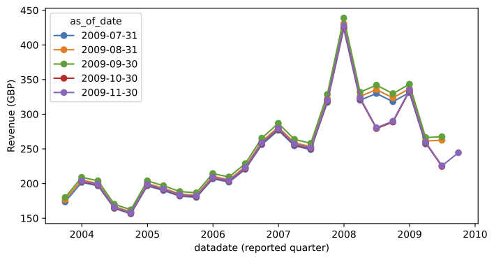
Figure 1 below displays the quarterly revenues for a sample company in the dataset. Each line corresponds to a different snapshot, i.e. it represents the most recent information available at the time. We see that the historical data evolve over different snapshots, as new financial reports correct previous one. When training our models, we need to maintain the distinction between the two types of dates, and only train based information available before a prediction.
The first modeling decision is that I will not be considering the full history of the company as inputs. I will only use data from the previous year (4 quarters) from a particular as_of_date. Therefore, I can immediately filter the dataset down to the 4 most recent datadate values for every as_of_date, for every security. This reduces the size of the dataset by a factor of ~6.
2. Methodology
I consider three different models for revenue forecasting:
- 4-quarter moving average: This is a simple baseline model. Simply take the revenue of a given security over each of the next 4 quarters to be the average of the last 4, for every security.
- Ridge linear regression: Least squared error regression over a set of numeric features and one-hot encoded categorical features (see next section). An L2 error is added to the total error (Ridge) for regularization, i.e. to minimize the effects of colinearity between variables and penalize large coefficients.
- LightGBM: Gradient boosted regression trees model developed by Microsoft. This is a good choice for this particular assignment because:
- It supports categorical features with large cardinality. For example, the security id which has nearly 2000 different unique values, can be handled as a feature.
- It is able to handle missing values (NaNs). This is crucial; I will come back to this point in the next section.
- It is fast and efficient on weak hardware (like mine).
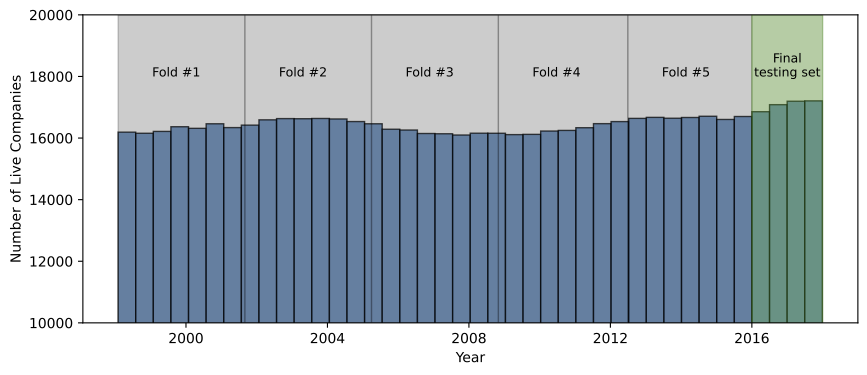
I evaluate and compare these models on a time-based cross-validation split. I hold out all data past 2016 as a final testing set. I manually divide the rest of the data into 5 “folds” which contain the same number of rows (note that this is slightly different from the classic time series split), which has folds of equal time duration. This split is illusrated in Figure 2 . To cross-validate, I train the models on fold 1, evaluate on 2. Then train on 1 and 2, evaluate on 3. Train on 1,2,3, evaluate on 4. Finally, train on 1,2,3,4, evaluate on 5. In this way, only data from the past is ever used to inform the model.
I repeated this cross-validation, modifying feature columns (acceptance threshold, number of lags, see next section), and experimenting with some of LightGBM’s hyperparameters (tree depth, learning rate, number of iteration). The final LightGBM model is then tested on the final testing set to report “official” performance metrics, which will be shown later.
The evaluation of models is based on two metrics: the mean squared error (MSE), and the mean absolute percent error (MAPE). For MAPE, we use a “safe” version which prevents the denominator (true revenues) from being zero or too small.
3. Feature Selection
3.1 Numeric Columns
- From price-related features, I only select
prccd_as_of_date_adj_GBP, the adjusted GBP price at theas_of_date. This is the most stable and comparable price metric across securities. - From fundamental buisness-related features, I include every quarterly feature (ends with the letter “q”), as long as it contains enough data. I set the threshold to 80% valid data (non-NaN) for the column to be included.
- I do not include any yearly features (ends with “y”). Most of them are just the cumulative quarterlies, and so it would be redundant to include them. For the yearly features that do not have a quarterly equivalent (e.g.
xidocy,rvy, tax-related columns), I found by inspection that their values were ambiguous, i.e. it was not clear if they were cumulatives or not. This matters; if they are cumulative, we would need to decumulate them to obtain true quarterly values. Because of this confusion, I decided not to include any of these columns. - I do not include the employees (emp) column. It has too many missing values.
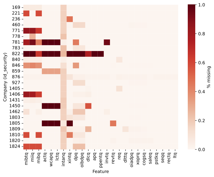
Note that many of these features have a lot of missing data by company. That is, while they pass the 80% valid data threshold overall, some individual security are well below the threshold. This is illustrated in Figure 3 below. While the feature columns are overall full enough, some companies (for example id 822 is a biggest offender) have a lot of missing data. This is a problem for the linear models, which cannot handle missing data. Therefore, for the linear fits, we simply filter them out. However, we keep all the missing values for the LightGBM model. This simplifies the modeling by a lot, as there is no need to impute values (which is always complicated an somewhat arbitrary). More importantly, missing values carry signal! For example, newer companies may not disclose a lot of information. The model can therefore potentially learn about the type of company from missing values.
3.2 Lagged features
\noindent For a subset of highly buisness-relevant quantities in the numeric columns selected from above, we also include 2 lagged features, i.e. the values from the two quarters preceding the latest datadate for a given as_of_date. This is how we encode the (recent) history of the company. The following features are included with lags:
- Revenue (
revtq) - Income (
ibq) - Assets (
atq) - Liquidity (
cheq) - Expenses (
xoprq)
3.3 Categorical columns
- I include the industry/sector code (
GICS_code_prefix), of which there are 11 unique values. This should encode information about how revenues differ from one industry to the other (say energy vs. technology). For the linear regression models, this variable is one-hot encoded. For example, an energy company hasis_sector_energy=1,is_sector_[anything_else]=0. - Only for the LightGBM model, I also include the security id, so that the model can learn about the behavior of individual companies, which should help refine the predictions.
3.4 Macroeconomic factors
Finally, I also include US macroeconomic indicator data. Here I made the assumption that all the companies were US-based, as the currency code in the dataset was uniformily USD. I downloaded data from the Federal Reserve Economic Data (FRED) from the past 30 years. Specifically, I included these indicators, for the following reasons:
- Unemployment rate (
UNRATE): The working population should affect revenues of all companies. - Oil price (
DCOILWTICO): Many companies in the dataset are in the energy sector, but also gas prices affect most companies expenses. - Real GDP growth (
GDPC1): Tracks the overall performance of the US economy. - Dollar index(
DTWEXM): How well the USD performs against other currencies. This affects trade, and therefore revenues. - Consumer price index (
CPIAUCSL): How much consumers are able to buy also affects revenues.
I resample these data on a quarterly basis, and then join them into the dataset, aligning with the as_of_date’s quarter. Importantly, I do not use any indicator values at the as_of_date, since these are typically not released at the moment of the snapshot. This would therefore constitute future information. Instead, I include the two previous quarters values for each indicator, as lagged columns.
4. Results
4.1 Model comparison on cross-validation
Table 1 displays the results of the cross-validation for all models and all data splits/folds. I show both MSE and MAPE, per quarter of forecast and overall. The fold column indicates the fold number of the validation set (with all previous folds used in training). I highlight in bold the best (lowest) MAPE scores for each quarter and overall. LightGBM has the best scores, and outperforms both Ridge regression and moving average for all quarters. The best model performance across all metrics was observed in the most recent fold (Fold 5), where data coverage and signal strength were likely highest.
The worst performing model is Ridge regression, by far. This can mean that the data is fundamentally non-linear or that the linear model is severely overfitted. In fact, both are probably true.
A curious result is the absurdely large MAPE numbers in Fold 1, across all models. I attribute this to quirks in the “burn-in” of training, fold 1 being the one with the smallest amount of data. Another possible factor is the presence of many companies with revenues near or equal to zero in the early years of the dataset. Because MAPE is a relative error, small true revenues in the denominator make it explode. Still, further investigation is needed…
| Model | Metric | Fold | Q1 | Q2 | Q3 | Q4 | Overall |
|---|---|---|---|---|---|---|---|
| Moving Avg | MSE | Fold 2 | 16440.78 | 25546.41 | 32038.48 | 38520.44 | 28136.53 |
| Fold 3 | 13650.70 | 16227.56 | 20445.79 | 23957.13 | 18570.29 | ||
| Fold 4 | 10495.69 | 11282.78 | 14451.92 | 16584.70 | 13203.77 | ||
| Fold 5 | 19444.42 | 21935.93 | 28872.73 | 35398.88 | 26412.99 | ||
| MAPE | Fold 2 | 662.456 | 1148.459 | 1466.858 | 1956.563 | 1308.584 | |
| Fold 3 | 0.209 | 0.235 | 0.269 | 0.292 | 0.251 | ||
| Fold 4 | 0.176 | 0.189 | 0.220 | 0.243 | 0.207 | ||
| Fold 5 | 0.180 | 0.192 | 0.228 | 0.258 | 0.215 | ||
| Ridge | MSE | Fold 2 | 146917.73 | 75390.22 | 39817.86 | 401815.58 | 165985.35 |
| Fold 3 | 13352.01 | 25167.69 | 34764.18 | 40072.48 | 28339.09 | ||
| Fold 4 | 17723.63 | 20465.20 | 13774.35 | 16466.57 | 17107.44 | ||
| Fold 5 | 11693.09 | 13155.19 | 15392.09 | 20686.60 | 15231.74 | ||
| MAPE | Fold 2 | 4023.028 | 12226.701 | 8301.897 | 67422.099 | 22993.431 | |
| Fold 3 | 0.570 | 0.929 | 1.251 | 1.273 | 1.006 | ||
| Fold 4 | 0.700 | 0.669 | 0.518 | 0.460 | 0.587 | ||
| Fold 5 | 0.278 | 0.360 | 0.401 | 0.390 | 0.357 | ||
| LightGBM | MSE | Fold 2 | 16985.78 | 20708.14 | 28734.98 | 20723.94 | 21788.21 |
| Fold 3 | 34516.93 | 34585.22 | 39274.37 | 41732.88 | 37527.35 | ||
| Fold 4 | 13653.61 | 21463.40 | 18735.62 | 20443.52 | 18574.04 | ||
| Fold 5 | 29990.21 | 38761.99 | 40455.55 | 57295.80 | 41625.88 | ||
| MAPE | Fold 2 | 866.391 | 2156.369 | 3009.078 | 3543.643 | 2393.870 | |
| Fold 3 | 0.268 | 0.281 | 0.279 | 0.307 | 0.284 | ||
| Fold 4 | 0.204 | 0.238 | 0.242 | 0.249 | 0.233 | ||
| Fold 5 | 0.175 | 0.189 | 0.198 | 0.232 | 0.198 |
4.2 LightGBM model performance on testing set
Finally, we evaluate the model’s performance on the test set (data from 2016 onwards). The results are in Table 2. Here are the main conclusions about the model’s performance:
- Overall MAPE on test set is 0.211, which is competitive with the best validation fold (Fold 4: 0.198). This means the model is not overfitted to the cross-validation set. We have a good proxy for how the model would perform in the real world.
- Quarterly MAPE is consistent (ranging from 0.198 to 0.227), indicating the model generalizes well across short- and medium-term forecasting.
- The root of the MSE (RMSE) error brings the error back to GBP scale. The overall RMSE is 129.5 million GBP
- The overall improvement to the baseline in a few percent at best. This data is difficult to forecast!
| Set | Metric | Q1 | Q2 | Q3 | Q4 | Overall |
|---|---|---|---|---|---|---|
| Test (all folds in training) | MSE | 16095.23 | 16688.62 | 16785.69 | 16182.42 | 16437.99 |
| MAPE | 0.227 | 0.211 | 0.198 | 0.208 | 0.211 |
5. Final portfolio building considerations
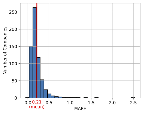
When building a portfolio based on revenue forecast, we want to know how well our model performs for different companies. There is a risk associated with the model performance. For a minimum risk portofolio, we may opt to only select companies in which the ML model performs well.
In fact, there is a lot of variance in the performance of the model when grouping by companies. I show the distribution of MAPE errors in Figure 4. We see that there are in fact many companies with much lower MAPE than the overall result. For example, these id’s have MAPE’s less than 5%: 93 , 95 , 694, 876, 879, 1177 , 1273 , 1595 , 1648 , 1682 , 1865. There are also a few outliers for which the model does not work at all! We probably would not want to include these in our portoflio.